Querying or Reading Data
OpenTSDB offers a number of means to extract, manipulate and analyze data. Data can be queried via CLI tools, an HTTP API and viewed as a GnuPlot graph. Open source tools such as Grafana and Bosun can also access TSDB data. Querying with OpenTSDB's tag based system can be a bit tricky so read through this document and checkout the following pages for deeper information. Example queries on this page follow the HTTP API format.
This page offers a quick overview of the typical query components. For details on each component, see the page referred to in the text or the table of contents above.
Query Components
OpenTSDB provides a number of tools and endpoints allowing for various query specifications that have evolved over time. The original syntax allowed for simple filtering, aggregation and downsampling. Later versions added support for functions and expressions. In general, each query has the following components:
| Parameter | Date Type | Required | Description | Example |
|---|---|---|---|---|
| Start Time | String or Integer | Required | Starting time for the query. This may be an absolute or relative time. See Dates and Times for details | 24h-ago |
| End Time | String or Integer | Optional | An end time for the query. If the end time is not supplied, the current time on the TSD will be used. See Dates and Times for details. | 1h-ago |
| Metric | String | Required | The full name of a metric in the system. Must be the complete name and it is always case sensitive | sys.cpu.user |
| Aggregation Function | String | Required | A mathematical function to use in combining multiple time series (i.e. how to merge time series in a group) | sum |
| Filter | String | Optional | Filters on tag values to reduce the number of time series picked up in a query or group and aggregate on various tags. | host=*,dc=lax |
| Downsampler | String | Optional | An optional interval and function to reduce the number of data points returned across time | 1h-avg |
| Rate | String | Optional | An optional flag to calculate the rate of change, per second, for the result | rate |
| Functions | String | Optional | Data manipulation functions such as additional filtering, time shifting, etc. | highestMax(...) |
| Expressions | String | Optional | Data manipulation functions across time series such as dividing one series by another. | (m2 / (m1 + m2)) * 100 |
Times
Absolute time stamps are supported in human readable format or Unix style integers. Relative times may be used for refreshing dashboards. Currently, all queries are able to cover a single time span. In the future we hope to provide an offset query parameter that would allow for aggregations or graphing of a metric over different time periods, such as comparing last week to 1 year ago. See Dates and Times for details on what is permissible.
While OpenTSDB can store data with millisecond resolution, by default, queries will return the data with second resolution to provide backwards compatibility for existing tools. If you are storing multiple data points per second, make sure that any query you issue includes a 1s-<func> downsampler to read the right data. Otherwise an indeterminate value will be emitted.
To extract data with millisecond resolution, use the /api/query endpoint and specify the msResolution (ms is also okay, but not recommended) JSON parameter or query string flag and it will bypass down sampling (unless specified) and return all timestamps in Unix epoch millisecond resolution. Also, the scan command line utility will return the timestamp as written in storage.
Filters
Every time series is comprised of a metric and one or more tag name/value pairs. In OpenTSDB, filters are applied against tag values (at this time TSDB does not provide filtering on metrics or tag keys). Since filters are optional in queries, if you request only the metric name, then every metric with any number or value of tags will be returned in the aggregated results. Filters are similar to the predicates following a WHERE clause in SQL. For example, if we have a stored data set:
sys.cpu.user host=webserver01,cpu=0  1356998400  1
sys.cpu.user host=webserver01,cpu=1  1356998400  4
sys.cpu.user host=webserver02,cpu=0  1356998400  2
sys.cpu.user host=webserver02,cpu=1  1356998400  1
and craft a simple query with the minimum requirements of a start time, aggregator and metric such as: start=1356998400&m=sum:sys.cpu.user, we will get a value of 8 at 1356998400 that aggregates and groups all 4 time series into one.
If we want to zoom into a particular series or set of series, we can use filters. For example, we can filter on the host tag via: start=1356998400&m=sum:sys.cpu.user{host=webserver01}. This query will return a value of 5, incorporating only the time series where host=webserver01. To drill down to a specific time series, you must include all of the tags for the series, e.g. the query start=1356998400&m=sum:sys.cpu.user{host=webserver01,cpu=0} will return 1.
Note
Inconsistent tags can cause unexpected results when querying. See Writing Data for details. Also see Explicit Tags below.
Read the Query Filters documentation for details.
Aggregation
A powerful feature of OpenTSDB is the ability to perform on-the-fly aggregations of multiple time series into a single set of data points. The original data is always available in storage but we can quickly extract the data in meaningful ways. Aggregation functions are means of merging two or more data points for a single time stamp into a single value.
Note
OpenTSDB aggregates data by default and requires an aggregation operator for every query. Each aggregator has to handle missing or data points at different time stamps for multiple series. This is performed via interpolation and can lead to unexpected results at query time if users are unaware of what TSDB is doing.
See Aggregation for details.
Downsampling
OpenTSDB can ingest a large amount of data, even a data point every second for a given time series. Thus queries may return a large number of data points. Accessing the results of a query with a large number of points from the API can eat up bandwidth. High frequencies of data can easily overwhelm Javascript graphing libraries, hence the choice to use GnuPlot. Graphs created by the GUI can be difficult to read, resulting in thick lines such as the graph below:
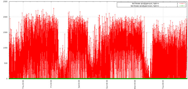
Downsampling can be used at query time to reduce the number of data points returned so that you can extract better information from a graph or pass less data over a connection. Down sampling requires an aggregation function and a time interval. The aggregation function is used to compute a new data point across all of the data points in the specified interval with the proper mathematical function. For example, if the aggregation sum is used, then all of the data points within the interval will be summed together into a single value. If avg is chosen, then the average of all data points within the interval will be returned.
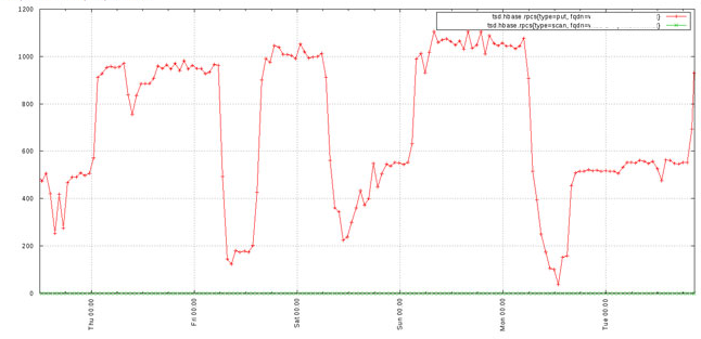
Using downsampling we can cleanup the previous graph to arrive at something much more useful:
For details, see Downsampling.
Rate
A number of data sources return values as constantly incrementing counters. One example is a web site hit counter. When you start a web server, it may have a hit counter of 0. After five minutes the value may be 1,024. After another five minutes it may be 2,048. The graph for a counter will be a somewhat straight line angling up to the right and isn't always very useful. OpenTSDB provides a rate conversion function that calculates the rate of change in values over time. This will transform counters into lines with spikes to show you when activity occurred and can be much more useful.
The rate is the first derivative of the values. It's defined as (v2 - v1) / (t2 - t1) where the times are in seconds. Therefore you will get the rate of change per second. Currently the rate of change between millisecond values defaults to a per second calculation.
OpenTSDB 2.0 provides support for special monotonically increasing counter data handling including the ability to set a "rollover" value and suppress anomalous fluctuations. When the counterMax value is specified in a query, if a data point approaches this value and the point after is less than the previous, the max value will be used to calculate an accurate rate given the two points. For example, if we were recording an integer counter on 2 bytes, the maximum value would be 65,535. If the value at t0 is 64000 and the value at t1 is 1000, the resulting rate per second would be calculated as -63000. However we know that it's likely the counter rolled over so we can set the max to 65535 and now the calculation will be 65535 - t0 + t1 to give us 2535.
Systems that track data in counters often revert to 0 when restarted. When that happens and we could get a spurious result when using the max counter feature. For example, if the counter has reached 2000 at t0 and someone reboots the server, the next value may be 500 at t1. If we set our max to 65535 the result would be 65535 - 2000 + 500 to give us 64035. If the normal rate is a few points per second, this particular spike, with 30s between points, would create a rate spike of 2,134.5! To avoid this, we can set the resetValue which will, when the rate exceeds this value, return a data point of 0 so as to avoid spikes in either direction. For the example above, if we know that our rate almost never exceeds 100, we could configure a resetValue of 100 and when the data point above is calculated, it will return 0 instead of 2,134.5. The default value of 0 means the reset value will be ignored, no rates will be suppressed.
Order of Operations
Understanding the order of operations is important. When returning query results the following is the order in which processing takes place:
- Filtering
- Grouping
- Downsampling
- Interpolation
- Aggregation
- Rate Conversion
- Functions
- Expressions